Let’s understand CNNs with an example –
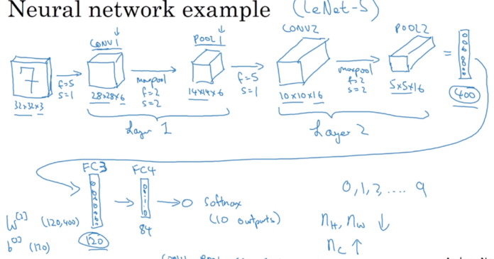
Figure 1. CNN Example – Source: Coursera DL Specialization
Let’s say you have a 32×32 image of digits from 0 to 10 with 3 channels (RGB). You pass it through a filter of size f in the 1st Convolutional Layer (CL1).
What is the size of the output image of the filter?
The size of the output image is calculated by the following formula:
 |
| Source: Medium |
In our case, let’s assume padding is 0 and stride is 1. The above formula results in output size of 28×28 for both the height and width of the image. Alright that’s a good start! Let’s keep going.
Notice the dimension 6 on the output of Layer 1.
Where do we get the third dimension from?
The third dimension is nothing but the number of filters in the layer. Given a filter of size f. There are #f number of filters in the layer and the dimension of EACH filter is of dimension f x f x nc
Where nc is number of channels/volume in the previous layer. In case of the first layer, the previous layer has 3 channels.
Now, If there are 6 such filters in layer 1 each filter produces a nout x nout x 1 output and given we have 6 filters – the output of Convolutional Layer 1 is nout x nout x 6.
What does Max Pooling do?
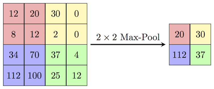
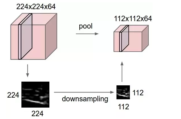
Pooling is a method of compressing information, think of high pixel values as more information and low pixel values as less information. Max Pooling is used to pick the maximum element in the filter’s window when convolved over the output of the previous layer.
 |
| Source: ComputerScienceWiki |
Figure 2. CNN Structure Summary – Source: Coursera DL Specialization
As you can observe, the activation size of the Network reduces gradually where you are down to 10 activations at the output of the Softmax to classify numbers from 0 to 9 and the number of parameters are significantly less than what it would have been if we were to implement this classifier with all layers as Fully connected.
More Readings:
http://cs231n.github.io/convolutional-networks/


